Calculating Gravity from Topographic Raster Data

In this post, I present a reproduction of the Harmonica tutorial Gravitational effect of topography, implemented in the notebook gravity_from_topography.ipynb, using a Digital Elevation Model (DEM) sourced from Colombia en Mapas.

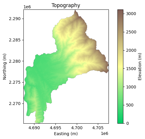
Topography Data: Digital Elevation Model (DEM)

A Digital Elevation Model (DEM) is a digital representation of the land surface’s elevation. The DEM used in this post is sourced from Colombia en Mapas and represents a specific region of Colombia. Using this elevation data, we can create a 3D model of the terrain and assign a specific density to the topography to compute its gravitational effect. For this, we can use the Harmonica Python library. The tutorial Gravitational effect of topography provides the code that serves as our guide.

1. Importing the DEM Data

We can use the Xarray Python library to import the DEM data and the rasterio engine to load the TIFF file:

import xarray as xr
filename = '../data/DEM_region_A.tif' # DTM taken from colombiaenmapas.gov.co
topography = xr.load_dataset(filename, engine="rasterio")

Next, we sort the data by coordinates in ascending order, as required by the forward modeling function in Harmonica that we will use later on:

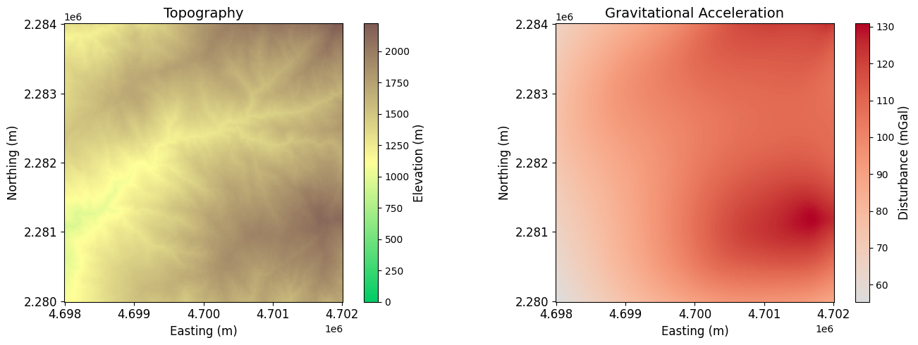
topography = topography.sortby(['x', 'y'])

Finally, we can plot the elevation map:

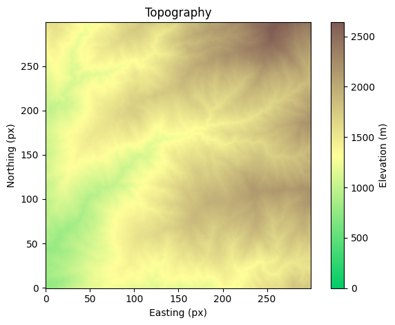
2. Domain for forward modelling

Next, we select the domain where the topography affects the measurements. The limits must correspond to the coordinate type of the dataset:

region = (4.697e6, 4.703e6, 2.279e6, 2.285e6)
topography_domain = topography.sel(
    x=slice(*region[:2]),
    y=slice(*region[2:]),
)

2.1 Subsampling the domain

We can subsample the domain to reduce computational load:

sampling = 10
topography_domain_subsampled = topography_domain.isel(
    x=slice(None, None, sampling),
    y=slice(None, None, sampling)
)

Next, we extract the elevation data from the dataset, which we call surface, and assign a density value to each spatial point. Following the Gravitational effect of topography tutorial, we set the terrain density to 2670 kg/m³ and assign the ocean a density contrast of -1900 kg/m³, calculated as the difference between water (1000 kg/m³) and the normal upper crust density (2900 kg/m³):

# elevation surface
surface = topography_domain_subsampled.band_data[0, :, :]
surface = surface.fillna(0)

# density model
density = 2670.0 * np.ones_like(surface)
density = np.where(surface >= 0, density, 1000 - 2900)

3. Select region of interest (or measurements points)

Then, we select the measurement points where the gravitational effect will be computed:

# Region to define the region of interest (ROI)
reduction = 2000
region_ROI = tuple(
	val + reduction 
	if i % 2 == 0 else val - reduction 
	for i, val in enumerate(region)
)

# Grid coordinates for the ROI
spacing = 20
coordinates_ROI = vd.grid_coordinates(region=region_ROI, spacing=spacing)

# Interpolate the surface to the measurement points
x = topography_domain_subsampled.x
y = topography_domain_subsampled.y
surface_interpolated = RectBivariateSpline(x, y, surface.T)
surface_ROI = surface_interpolated.ev(coordinates_ROI[0], coordinates_ROI[1])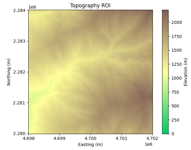

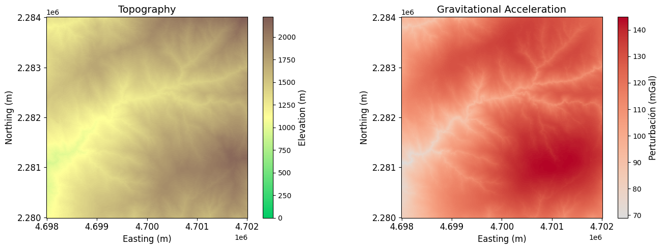
4. Calculate gravity

Following the Gravitational effect of topography tutorial, we use the harmonica.prism_layer function to create a 3D model of the terrain with the specified density. Then, we compute its gravitational effect at the observation points using harmonica.prism_gravity.

4.1 Observation points at the surface

# Create prisms from topography
prisms = hm.prism_layer(
    coordinates=(x, y),
    surface=surface,
    reference=0,
    properties={"density": density},
)

# Compute gravity at the measurement points
extra_coords = surface_ROI
prisms_gravity = prisms.prism_layer.gravity(
	(coordinates_ROI[0], coordinates_ROI[1], extra_coords), 
	field="g_z"
)

4.2 Observation points at 2200 meters

# Compute gravity at the measurement points
extra_coords = 2200 * np.ones_like(coordinates_ROI[0])
prisms_gravity = prisms.prism_layer.gravity(
	(coordinates_ROI[0], coordinates_ROI[1], extra_coords), 
	field="g_z"
)

As the observation height increases, the magnitude of the gravitational disturbance decreases, and the fine details in the signal become less pronounced. This effect occurs because the gravitational field weakens with distance from the mass sources, leading to a smoother and lower-contrast anomaly pattern.