Accessing DEMs and Sentinel-1 Data from the Planetary Computer catalogs

Blog

Lineament Detection

October 5, 2025·

JulianSoZa

alejaboterob

nicoguaro

In this post, I reproduce the process of obtaining satellite data from the Microsoft Planetary Computer, focusing on Digital Elevation Models (DEMs) and Synthetic Aperture Radar (SAR) imagery. I also show how to access, visualize, and combine multiple items. The code examples DEM_getting.ipynb and sentinel-1_GRD_getting.ipynb are based on the official Microsoft Planetary Computer documentation: Reading Data from the STAC API.

Libraries

We’ll use the following Python libraries, including planetary_computer and pystac for accessing and managing data assets.

import matplotlib.pyplot as plt
import xarray as xr
import pystac
import planetary_computer
import rioxarray
import numpy as np
import rasterio
from rasterio.merge import merge

Accessing an individual item’s data assets

DEMs

The Planetary Computer platform provides code examples for retrieving an item’s data assets:

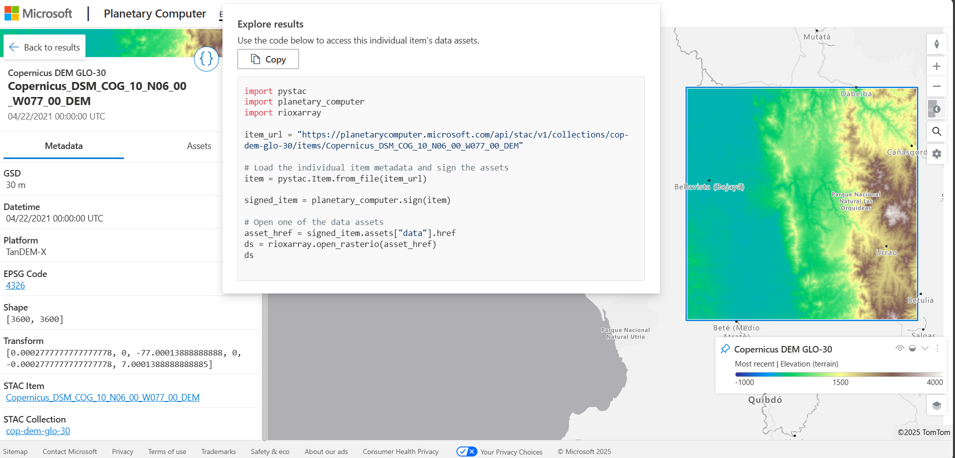
planetary_computer_single_item — Screenshot taken from Planetary Computer

item_url = "https://planetarycomputer.microsoft.com/api/stac/v1/collections/cop-dem-glo-30/items/Copernicus_DSM_COG_10_N06_00_W077_00_DEM" # item 1
# item_url = "https://planetarycomputer.microsoft.com/api/stac/v1/collections/cop-dem-glo-30/items/Copernicus_DSM_COG_10_N06_00_W078_00_DEM" # item 2

# Load the individual item metadata and sign the assets
item = pystac.Item.from_file(item_url)

signed_item = planetary_computer.sign(item)

# Open one of the data assets 
asset_href = signed_item.assets["data"].href
ds = rioxarray.open_rasterio(asset_href)

We can then plot the DEM data:

plt.figure()
plt.imshow(ds[0, ...], cmap=cmap_terrain_crust, vmin=0, vmax=4500)
plt.colorbar()
plt.show()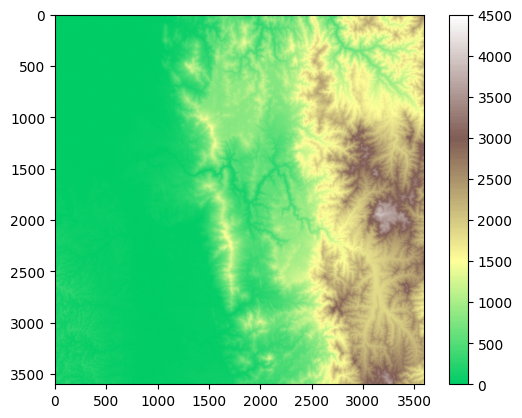

DEM_single_item — Data taken from Planetary Computer

SARs

To access a Sentinel-1 SAR dataset:

item_url = "https://planetarycomputer.microsoft.com/api/stac/v1/collections/sentinel-1-grd/items/S1C_IW_GRDH_1SDV_20250922T232209_20250922T232234_004244_0086B0" # item 1

# item_url = "https://planetarycomputer.microsoft.com/api/stac/v1/collections/sentinel-1-grd/items/S1C_IW_GRDH_1SDV_20250922T232144_20250922T232209_004244_0086B0" # item 2

# Load the individual item metadata and sign the assets
item = pystac.Item.from_file(item_url)

signed_item = planetary_computer.sign(item)

# Open one of the data assets (other asset keys to use: 'vv')
asset_href = signed_item.assets["vh"].href
ds = rioxarray.open_rasterio(asset_href)

Reproject the raster to a CRS:

ds_reprojected = ds.rio.reproject("EPSG:4326")

And save it as a GeoTIFF (compatible with GIS software):

filename = '../../data/SAR/sentinel-1_GRD_VH_1.tif'
ds_reprojected.rio.to_raster(filename)

If the dataset is very large, you can subsample it:

sampling = 10
SAR = ds_reprojected.isel(
    x=slice(None, None, sampling),
    y=slice(None, None, sampling)
)

And plot the subsampled data:

raster_plotting.plot_raster_data(SAR.x, SAR.y, SAR[0], vmax=400)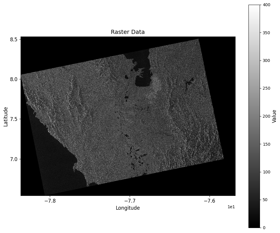

sentinel-1_GRD_single_item — Data taken from Planetary Computer

Combining two individual item’s data assets.

DEMs

If we already have the dataset ds for the first DEM item, we can combine it with another as follows:

item_url = "https://planetarycomputer.microsoft.com/api/stac/v1/collections/cop-dem-glo-30/items/Copernicus_DSM_COG_10_N06_00_W078_00_DEM" # item 2

item = pystac.Item.from_file(item_url)
signed_item = planetary_computer.sign(item)
asset_href = signed_item.assets["data"].href
ds2 = rioxarray.open_rasterio(asset_href)

# Ensure both datasets have CRS information
ds_crs = ds.rio.write_crs("EPSG:4326", inplace=False)
ds2_crs = ds2.rio.write_crs("EPSG:4326", inplace=False)

combined_ds = xr.combine_by_coords([ds_crs, ds2_crs])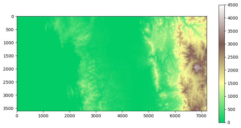

DEM_two_items — Data taken from Planetary Computer

SARs

We can merge two saved GeoTIFFs as follows:

# Paths to the GeoTIFF files to be mosaicked
tiff1 = '../../data/SAR/sentinel-1_GRD_VH_1.tif'
tiff2 = '../../data/SAR/sentinel-1_GRD_VH_2.tif'

# Open the files as rasterio objects
src_files_to_mosaic = []
for path in [tiff1, tiff2]:
    src = rasterio.open(path)
    src_files_to_mosaic.append(src)

Mosaic the rasters and define metadata:

# Mosaic the rasters
mosaic, out_trans = merge(src_files_to_mosaic)

# Copy metadata from the first raster
out_meta = src.meta.copy()
out_meta.update({
    "driver": "GTiff",
    "height": mosaic.shape[1],
    "width": mosaic.shape[2],
    "transform": out_trans
})

Finally, save the merged result:

with rasterio.open("../../data/SAR/sentinel-1_GRD_VH.tif", "w", **out_meta) as dest:
     dest.write(mosaic)

Reading Combined Dataset

filename = '../../data/SAR/sentinel-1_GRD_VH.tif'
SAR = rioxarray.open_rasterio(filename)

Optionally, sample and plot the result:

sampling = 10
SAR_sampled = SAR.isel(
    x=slice(None, None, sampling),
    y=slice(None, None, sampling)
)
raster_plotting.plot_raster_data(SAR_sampled.x, SAR_sampled.y, SAR_sampled[0], vmax=400)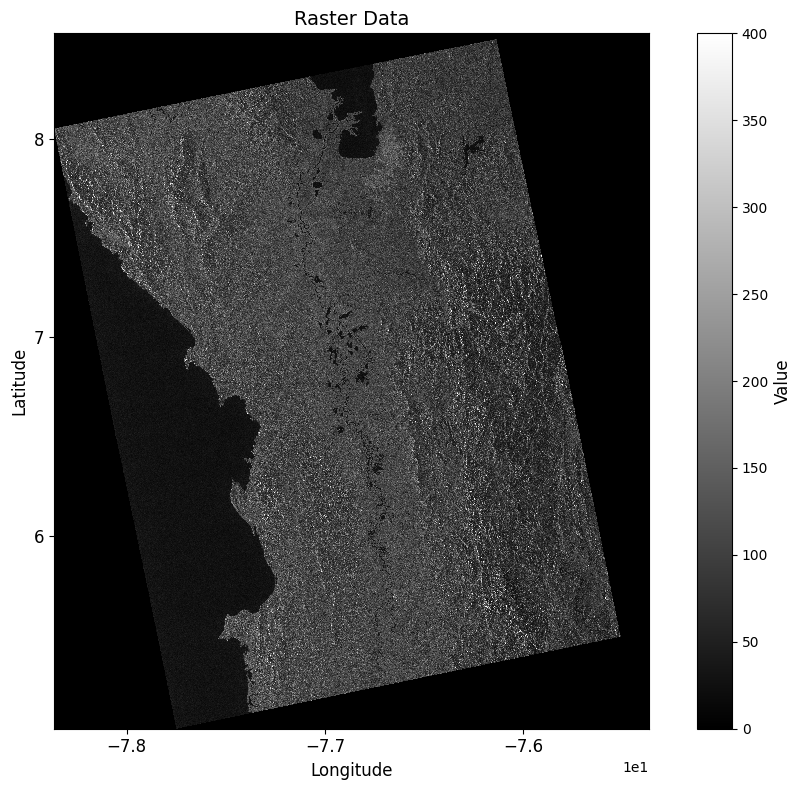

sentinel-1_GRD_mosaic — Data taken from Planetary Computer

Accessing Multiple Items

The Planetary Computer platform also provides methods for retrieving multiple data items by defining a search query.

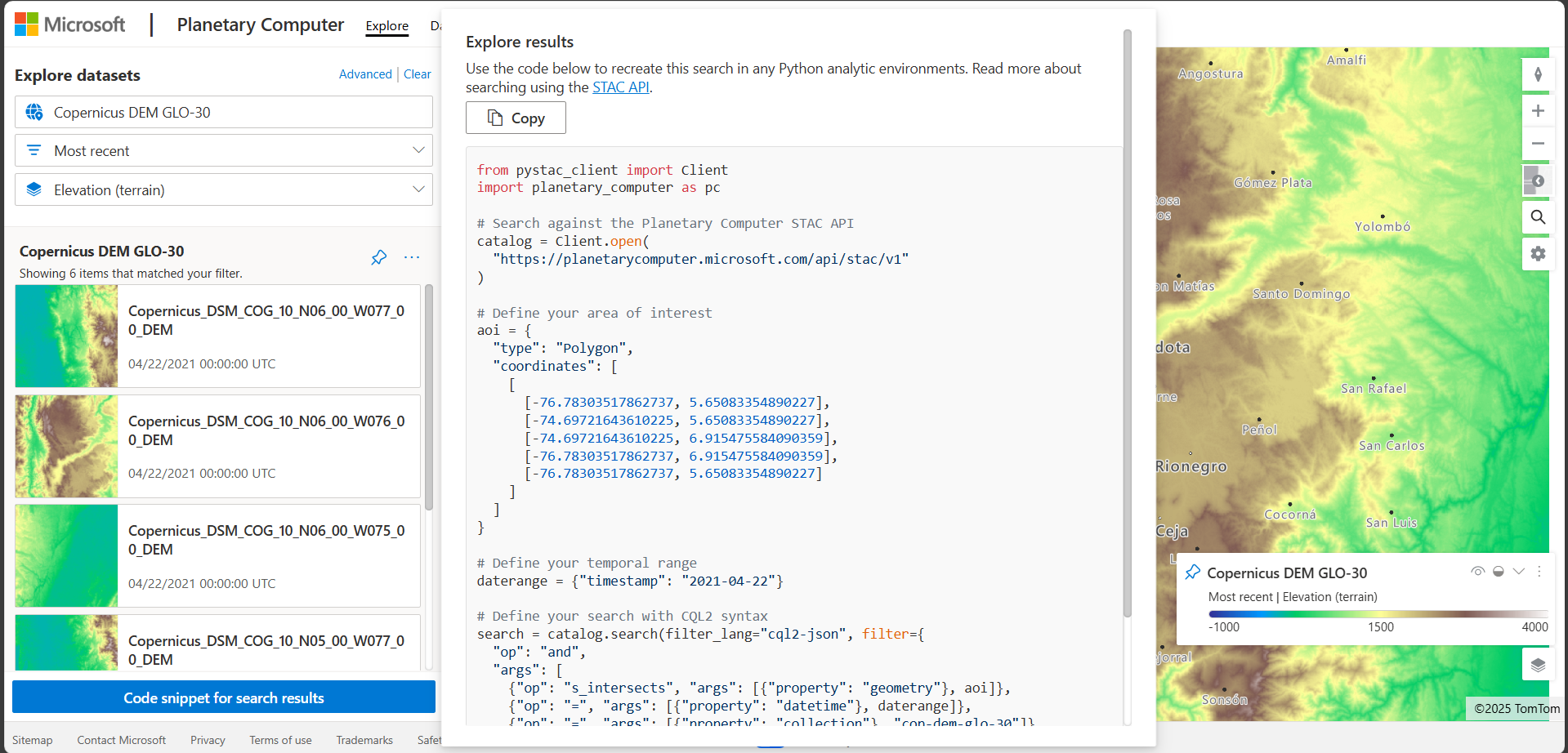
planetary_computer_multiple_items — Screenshot taken from Planetary Computer

from pystac_client import Client
import planetary_computer as pc

# Search against the Planetary Computer STAC API
catalog = Client.open(
  "https://planetarycomputer.microsoft.com/api/stac/v1",
  modifier=planetary_computer.sign_inplace,
)

# Define your area of interest
aoi = {
  "type": "Polygon",
  "coordinates": [
    [
      [-78, 5],
      [-76.5, 5],
      [-76.5, 8.5],
      [-78, 8.5],
      [-78, 5]
    ]
  ]
}

# Define your temporal range
daterange = {"timestamp": "2021-04-22"}

# Define your search with CQL2 syntax
search = catalog.search(filter_lang="cql2-json", filter={
  "op": "and",
  "args": [
    {"op": "s_intersects", "args": [{"property": "geometry"}, aoi]},
    {"op": "=", "args": [{"property": "datetime"}, daterange]},
    {"op": "=", "args": [{"property": "collection"}, "cop-dem-glo-30"]}
  ]
})
items = search.item_collection()
print("Number of items found:", len(items))

Number of items found: 10

Now, we can load the DEM tiles that we want to select, in this case we load all of them:

dem_arrays = []

for i, item in enumerate(items):
    print(f"Loading item {i+1}/{len(items)}: {item.id}")
    
    # open the DEM tile
    dem_tile = rioxarray.open_rasterio(item.assets["data"].href)
    
    # CRS information
    dem_tile_crs = dem_tile.rio.write_crs("EPSG:4326", inplace=False)
    
    # append to list
    dem_arrays.append(dem_tile_crs)

print(f"Loaded {len(dem_arrays)} DEM tiles")

Loading item 1/10: Copernicus_DSM_COG_10_N08_00_W078_00_DEM
Loading item 2/10: Copernicus_DSM_COG_10_N08_00_W077_00_DEM
Loading item 3/10: Copernicus_DSM_COG_10_N07_00_W078_00_DEM
Loading item 4/10: Copernicus_DSM_COG_10_N07_00_W077_00_DEM
Loading item 5/10: Copernicus_DSM_COG_10_N06_00_W078_00_DEM
Loading item 6/10: Copernicus_DSM_COG_10_N06_00_W077_00_DEM
Loading item 7/10: Copernicus_DSM_COG_10_N05_00_W078_00_DEM
Loading item 8/10: Copernicus_DSM_COG_10_N05_00_W077_00_DEM
Loading item 9/10: Copernicus_DSM_COG_10_N04_00_W078_00_DEM
Loading item 10/10: Copernicus_DSM_COG_10_N04_00_W077_00_DEM
Loaded 10 DEM tiles

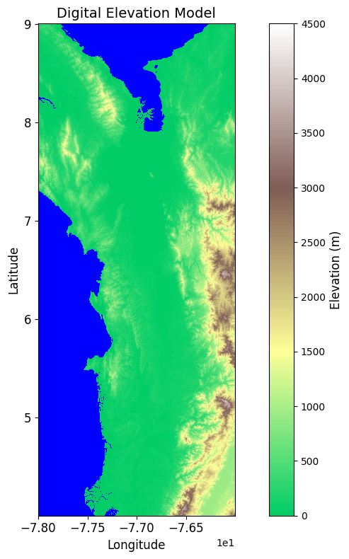
And finally, combine all tiles into a single dataset:

# Combine all DEM tiles into a single xarray DataArray
print("Combining DEM tiles...")
combined_dem = xr.combine_by_coords(dem_arrays)
print(f"Combined DEM shape: {combined_dem.shape}")
print(f"Combined DEM bounds: x({combined_dem.x.values.min():.4f}, {combined_dem.x.values.max():.4f}), y({combined_dem.y.values.min():.4f}, {combined_dem.y.values.max():.4f})")
combined_dem;

Combining DEM tiles...
Combined DEM shape: (1, 18000, 7200)
Combined DEM bounds: x(-78.0000, -76.0003), y(4.0003, 9.0000)

DEM_read — Data taken from Planetary Computer

Calculating Gravity from Topographic Raster Data Training a Convolutional Neural Network (CNN) with a Fault Mapping Dataset for Linear Structure Detection