Helmholtz Equation - Finite Differences


In this post, I show the finite difference scheme of the Helmholtz Equation for a 2D domain and its Dirichlet-condition version. The code developed in dirichlet_conditions.py calculates the numerical solution using this methodology.
Finite Difference Method: Central Scheme
First Derivate
$$ f'(x) \approx \frac{f(x+h) - f(x-h)}{2h} = \frac{f_{i+1} - f_{i-1}}{2\Delta x}$$Second Derivate
$$ f''(x) \approx \frac{f(x+h) - 2f(x) + f(x-h)}{h^2} = \frac{f_{i+1} - 2f_{i} + f_{i-1}}{\Delta x^2} $$Helmholtz Equation
The 2D Helmholtz equation for a field $u(x,z)$, with wavenumber $k$ and source term $s(x,z)$, is
$$ \left(\nabla^2 + k^2\right) u(x,z) = s(x,z), $$where $\nabla^2$ is the 2D Laplacian operator. In Cartesian coordinates, this can be written as
$$ \frac{\partial^2 u(x,z)}{\partial x^2} + \frac{\partial^2 u(x,z)}{\partial z^2} + k^2 u(x,z) = s(x,z). $$Here, $x$ represents the horizontal coordinate (parallel to the surface in geophysical applications), and $z$ represents the vertical or depth coordinate.
Finite Difference Discretization
Using the central difference scheme for the second derivative, we can discretize the Helmholtz equation as follows:
$$ \frac{u_{i+1,j} - 2u_{i,j} + u_{i-1,j}}{\Delta x^2} + \frac{u_{i,j+1} - 2u_{i,j} + u_{i,j-1}}{\Delta z^2} + k^2 u_{i,j} = s_{i,j}, $$where $i$ and $j$ are the discretization indices for the $x$ and $z$ coordinates, respectively.
We can now use the SymPy Python package to organize this expression and collect the terms corresponding to each node:
import sympy as sym

u_i_j, u_i1_j, u_1i_j, u_i_j1, u_i_1j = sym.symbols('u_{i\,j} u_{i+1\,j} u_{i-1\,j} u_{i\,j+1} u_{i\,j-1}')
k = sym.symbols('k')
s_i_j = sym.symbols('s_{i\,j}')

dx, dz = sym.symbols('Delta_x Delta_z')

expr = (  1/(dx**2) * (u_i1_j - 2*u_i_j + u_1i_j)
        + 1/(dy**2) * (u_i_j1 - 2*u_i_j + u_i_1j)
        + k**2 * u_i_j)

display(sym.Eq(expr, s_i_j))
$\displaystyle k^{2} u_{i,j} + \frac{u_{i,j+1} + u_{i,j-1} - 2 u_{i,j}}{\Delta_{z}^{2}} + \frac{u_{i+1,j} - 2 u_{i,j} + u_{i-1,j}}{\Delta_{x}^{2}} = s_{i,j}$
expr_terms_collected = sym.collect(sym.expand(expr), [u_i_j, u_i1_j, u_1i_j, u_i_j1, u_i_1j])
display(sym.Eq(expr_terms_collected, s_i_j))
$\displaystyle u_{i,j} \left(k^{2} - \frac{2}{\Delta_{z}^{2}} - \frac{2}{\Delta_{x}^{2}}\right) + \frac{u_{i,j+1}}{\Delta_{z}^{2}} + \frac{u_{i,j-1}}{\Delta_{z}^{2}} + \frac{u_{i+1,j}}{\Delta_{x}^{2}} + \frac{u_{i-1,j}}{\Delta_{x}^{2}} = s_{i,j}.$
Solution Methodology
Linear System
Now, we can construct a linear system from the discretized equation:
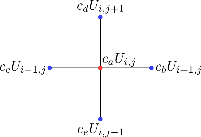
$$ c_a \, u_{i,j} + c_b \, u_{i+1,j} + c_c \, u_{i-1,j} + c_d \, u_{i,j+1} + c_e \, u_{i,j-1} = s_{i,j}, $$with the following coefficients:
$$ c_a = k^2 - \frac{2}{\Delta x^2} - \frac{2}{\Delta z^2}, \quad c_b = c_c = \frac{1}{\Delta x^2}, \quad c_d = c_e = \frac{1}{\Delta z^2}. $$Each node thus has a weight in the finite difference equation that determines its contribution to the linear system:
Domain with Dirichlet Conditions
For a problem defined on a domain with the following Dirichlet boundary conditions
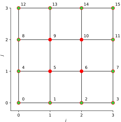 we can solve the corresponding linear matrix system:
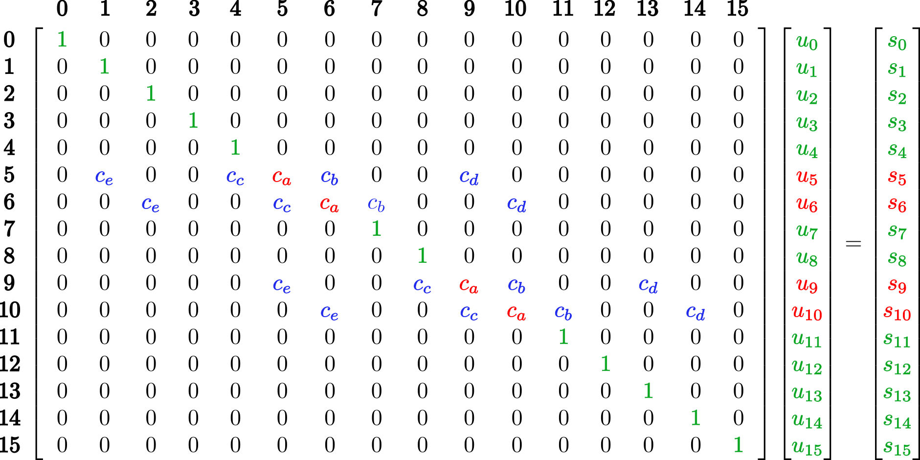
The code developed in dirichlet_conditions.py calculates the numerical solution using this methodology. The Python code constructs the linear matrix system by assigning the weights of each node to the system matrix. This results in a sparse matrix, which we create using the csr_matrix class from SciPy. The linear system is then solved efficiently using the spsolve function from SciPy.
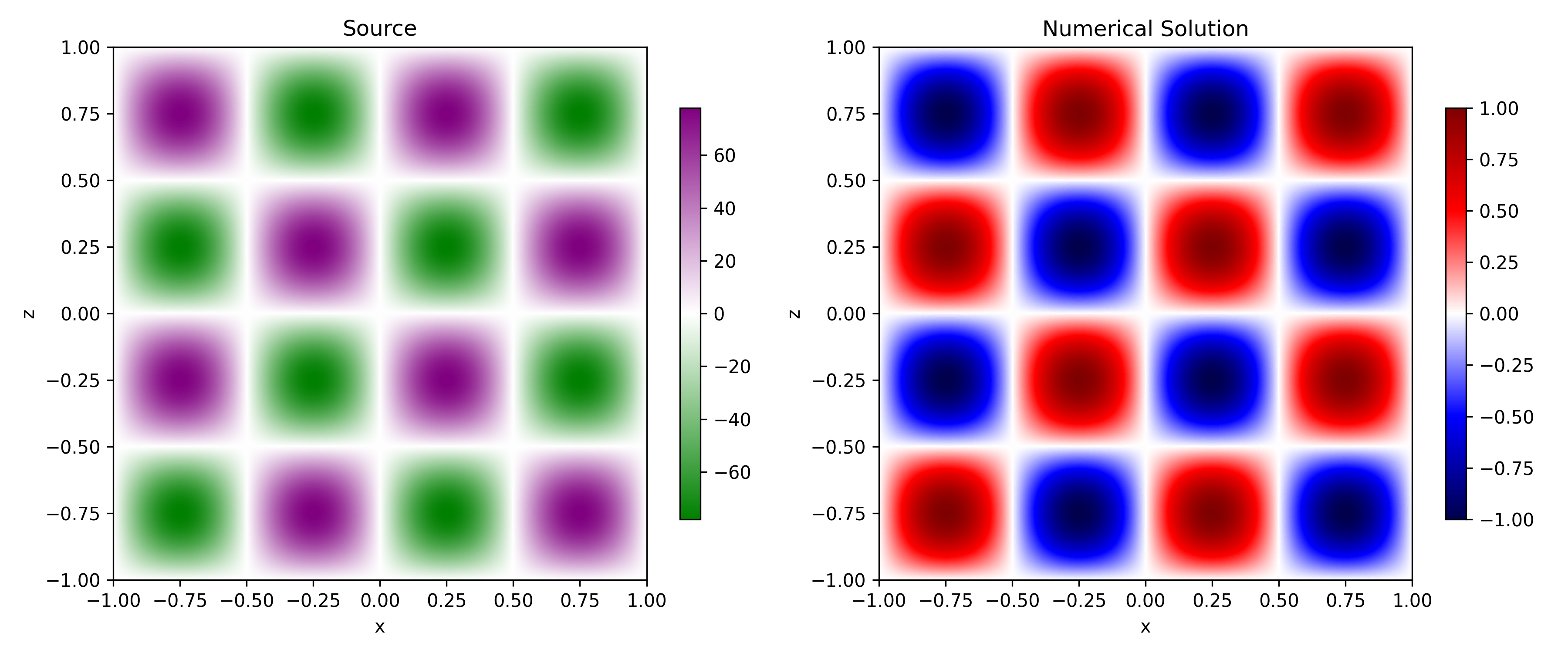
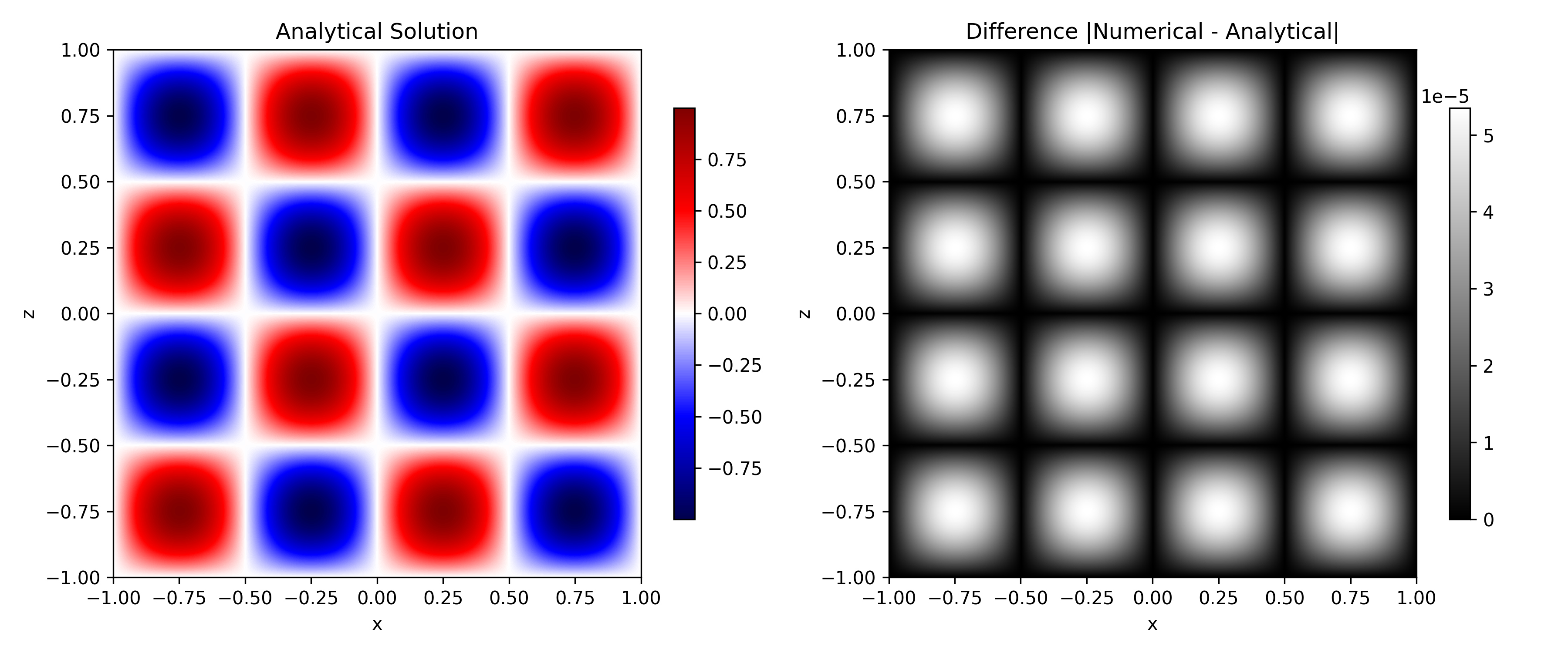
To assess the code, we simulated the following problem:
$$ \left(\nabla^2+k^2\right)u(x,z) = s(x,z), \quad \textbf{Helmholtz equation}$$$$ s(x,z) = \left[-(a_x \pi)^2 - (a_z \pi)^2 + k^2\right]\sin(a_x \pi x) \sin(a_z \pi z), \quad \textbf{Source}$$$$x,z \in \Omega = [-1,\,1]\times[-1,\,1], \quad \textbf{Rectangular domain}$$$$ u(x,z) = 0, \quad x,z \in \partial \Omega, \quad \textbf{Dirichlet boundary conditions}.$$The analytical solution for this problem is:
$$u(x,z) = \sin(a_x \pi x) \sin(a_z \pi z).$$For $a_x = a_z = 2$, the numerical solution agrees closely with the analytical solution, with a maximum absolute difference of $5.35 \times 10^{-5}$: