Helmholtz Equation, Finite Differences and PML Boundary Conditions

In this post, I present the finite difference formulation of the Helmholtz equation for a 2D domain with Perfectly Matched Layer (PML) boundary conditions. These boundary conditions allow us to simulate wave propagation in an effectively infinite medium by reducing artificial reflections at the computational boundaries. The code developed in pml_conditions.py calculates the numerical solution using this methodology..

Helmholtz Equation

The 2D Helmholtz equation for a field $u(x,z)$, with wavenumber $k$ and source term $s(x,z)$, is

where $\nabla^2$ is the 2D Laplacian operator. In Cartesian coordinates, this can be written as

Here, $x$ represents the horizontal coordinate (parallel to the surface in geophysical applications), and $z$ represents the vertical or depth coordinate.

Simulating an Infinite Domain

When simulating wave propagation in an infinite domain, it is common to truncate the wavefield to a finite computational domain due to the limited memory of computers. To minimize unwanted numerical reflections at the boundaries, Absorbing Boundary Conditions (ABC) or Perfectly Matched Layers (PML) are typically employed. The numerical solution should closely approximate the restriction of the true solution that would be obtained in the original infinite physical domain ^{1 2}.

Perfectly Matched Layer (PML)

A PML is an artificial dissipative zone that surrounds the computational domain, designed to strongly absorb outgoing waves without reflecting them back into the interior ¹. When using PML to simulate wavefields within a 2D rectangular domain, the Helmholtz equation can be expressed as:

where $k$ is the wavenumber, and

with $\omega$ the angular frequency and $\sigma$ a differentiable damping function used to absorb the wave energy within the PML boundaries ².

Outside of the PML, $\sigma_{x,z}=0$ . Meanwhile, inside of the PML, $\sigma_{x,z}$ are defined as

where:

• $a_0$ is a constant scaling coefficient,
• $f_0$ is the dominant source frequency,
• $L_{PML}$ is the physical thickness of the PML layer, and
• $l_{x,z}$ is the distance from point $(x, z)$ to the respective PML boundary.

This equation can be rewritten as:

and expanded as:

where $A = \frac{e_z}{e_x}$, $B = \frac{e_x}{e_z}$, and $C = e_x e_z k^2$.

Finite Difference Discretization

Using the central difference scheme for the second derivative, we can discretize the Helmholtz equation as follows:

$\displaystyle \frac{A_{i,j} \left(u_{i+1,j} - 2 u_{i,j} + u_{i-1,j}\right)}{\Delta_{x}^{2}} + \frac{B_{i,j} \left(u_{i,j+1} + u_{i,j-1} - 2 u_{i,j}\right)}{\Delta_{z}^{2}} + C_{i,j} u_{i,j} + \frac{\left(B_{i,j+1} - B_{i,j-1}\right) \left(u_{i,j+1} - u_{i,j-1}\right)}{4 \Delta_{z}^{2}} + \frac{\left(A_{i+1,j} - A_{i-1,j}\right) \left(u_{i+1,j} - u_{i-1,j}\right)}{4 \Delta_{x}^{2}} = s_{i,j},$

Here, $i$ and $j$ are the discretization indices for the $x$ and $z$ coordinates, respectively.

We can use the SymPy Python package to symbolically organize this expression and collect terms for each node:

import sympy as sym

u_i_j, u_i1_j, u_1i_j, u_i_j1, u_i_1j = sym.symbols('u_{i\,j} u_{i+1\,j} u_{i-1\,j} u_{i\,j+1} u_{i\,j-1}')

A_i_j, A_i1_j, A_1i_j = sym.symbols('A_{i\,j} A_{i+1\,j} A_{i-1\,j}')

B_i_j, B_i_j1, B_i_1j = sym.symbols('B_{i\,j} B_{i\,j+1} B_{i\,j-1}')

C_i_j = sym.symbols('C_{i\,j}')

s_i_j = sym.symbols('s_{i\,j}')

dx, dz = sym.symbols('Delta_x Delta_z')

expr = (  1/(2*dx) * (A_i1_j - A_1i_j) * 1/(2*dx) * (u_i1_j - u_1i_j)
        + A_i_j/(dx**2) * (u_i1_j - 2*u_i_j + u_1i_j)
        + 1/(2*dz) * (B_i_j1 - B_i_1j) * 1/(2*dz) * (u_i_j1 - u_i_1j)
        + B_i_j/(dz**2) * (u_i_j1 - 2*u_i_j + u_i_1j)
        + C_i_j * u_i_j)
          
display(sym.Eq(expr, s_i_j))

$\displaystyle \frac{A_{i,j} \left(u_{i+1,j} - 2 u_{i,j} + u_{i-1,j}\right)}{\Delta_{x}^{2}} + \frac{B_{i,j} \left(u_{i,j+1} + u_{i,j-1} - 2 u_{i,j}\right)}{\Delta_{z}^{2}} + C_{i,j} u_{i,j} + \frac{\left(B_{i,j+1} - B_{i,j-1}\right) \left(u_{i,j+1} - u_{i,j-1}\right)}{4 \Delta_{z}^{2}} + \frac{\left(A_{i+1,j} - A_{i-1,j}\right) \left(u_{i+1,j} - u_{i-1,j}\right)}{4 \Delta_{x}^{2}} = s_{i,j},$

expr_terms_collected = sym.collect(sym.expand(expr), [u_i_j, u_i1_j, u_1i_j, u_i_j1, u_i_1j])
display(sym.Eq(expr_terms_collected, s_i_j))

$\displaystyle u_{i+1,j} \left(\frac{A_{i+1,j}}{4 \Delta_{x}^{2}} + \frac{A_{i,j}}{\Delta_{x}^{2}} - \frac{A_{i-1,j}}{4 \Delta_{x}^{2}}\right) + u_{i,j+1} \left(\frac{B_{i,j+1}}{4 \Delta_{z}^{2}} - \frac{B_{i,j-1}}{4 \Delta_{z}^{2}} + \frac{B_{i,j}}{\Delta_{z}^{2}}\right) + u_{i,j-1} \left(- \frac{B_{i,j+1}}{4 \Delta_{z}^{2}} + \frac{B_{i,j-1}}{4 \Delta_{z}^{2}} + \frac{B_{i,j}}{\Delta_{z}^{2}}\right) + u_{i,j} \left(- \frac{2 A_{i,j}}{\Delta_{x}^{2}} - \frac{2 B_{i,j}}{\Delta_{z}^{2}} + C_{i,j}\right) + u_{i-1,j} \left(- \frac{A_{i+1,j}}{4 \Delta_{x}^{2}} + \frac{A_{i,j}}{\Delta_{x}^{2}} + \frac{A_{i-1,j}}{4 \Delta_{x}^{2}}\right) = s_{i,j}.$

Solution Methodology

Linear System

Now, we can construct a linear system from the discretized equation:

with the following coefficients:

The code developed in pml_conditions.py computes the numerical solution using a methodology similar to that described in Helmholtz Equation - Finite Differences. The Python code constructs the linear matrix system by assigning the weights of each node to the system matrix. This results in a sparse matrix, which we create using the csr_matrix class from SciPy. The linear system is then solved efficiently using the spsolve function from SciPy.

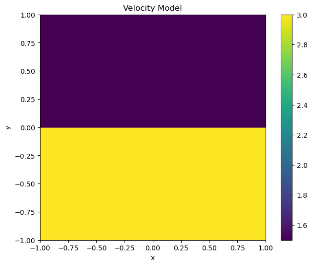
To evaluate the code, we simulated a problem similar to that presented in Wave Equation to Frequency Domain using Devito. The velocity model consists of a single interface separating two media:

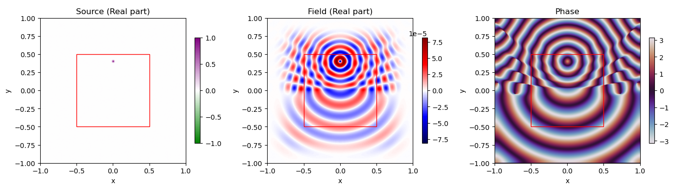
The following figure shows the numerical solution obtained for the full domain with PML conditions. The region outside the red square corresponds to the PML, while the inner region represents the main domain where the Helmholtz equation solution is sought:

Zooming into the main region, we obtain:

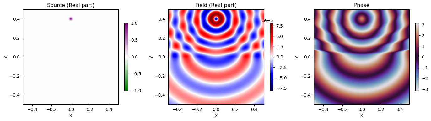
which corresponds to the solution obtained using Devito in Wave Equation to Frequency Domain using Devito.

References

F. Nataf, “Absorbing boundary conditions and perfectly matched layers in wave propagation problems,” in Direct and Inverse problems in Wave Propagation and Applications, De Gruyter, 2013. [Online]. Available: https://hal.science/hal-00799759v1 ↩︎ ↩︎
C. Song, T. Alkhalifah, and U. B. Waheed, “A versatile framework to solve the Helmholtz equation using physics-informed neural networks,” Geophys. J. Int., vol. 228, no. 3, pp. 1750–1762, Mar. 2022, doi: 10.1093/gji/ggab434. ↩︎ ↩︎