Wave Equation to Frequency Domain using Devito

In this post, I present a reproduction of the Devito ^{1 2} tutorial 17 – On-the-fly Discrete Fourier Transform, implemented in the notebook wave_eq_to_freq_domain.ipynb, where the frequency components of the wavefield are computed.

On-the-fly Fourier Transform

The discrete Fourier transform (DFT) is defined as:

where $X_k$ is the DFT of the sequence $x_n$, $N$ is the number of samples, $k$ is the frequency index and $n$ is the time index ³.

The DFT can be used to compute the frequency components of the wavefield as it propagates through the subsurface ³.

The key idea is to update the Fourier modes at each time step using the current wavefield values:

where $F_k(t)$ is the Fourier mode at frequency $\omega_k$ and time $t$, $u(t)$ is the wavefield at time $t$ and $\Delta t$ is the time step ³.

Model and Acquisition Geometry

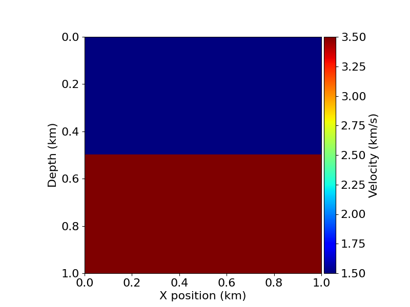
First, we define the dimensions of the physical domain and the parameters of the model, including:

• The velocity profile of wave propagation,
• The origin of the coordinate system,
• The number of discrete positions within the domain,
• The spatial grid spacing,
• and the boundary conditions.

In this case, we use one of the demo models provided by Devito, which employs perfectly matched layer (PML) boundary conditions to absorb outgoing waves and minimize reflections at the edges of the domain.

from devito import *
from examples.seismic import demo_model, AcquisitionGeometry
from examples.seismic import plot_velocity, TimeAxis, RickerSource
import numpy as np

# Model ----------------------------------
model = demo_model(
	'layers-isotropic',
	vp=3.0, 
	origin=(0., 0.), 
	shape=(201, 201), 
	spacing=(5., 5.), 
	nbl=150, 
	nlayers=2
	)
	
plot_velocity(model)
# ----------------------------------------

Then, we configure the acquisition geometry, i.e., the arrangement of sources and receivers.
In this case, a single source is positioned horizontally at the center of the model at a depth of $20 \ \text{m}$. We also define the time discretization, which determines the temporal resolution of the simulation.

# Acquisition geometry -------------------
# Source
# First, position source centrally in all dimensions, then set depth
src_coordinates = np.empty((1, 2))
src_coordinates[0, :] = np.array(model.domain_size) * .5
src_coordinates[0, -1] = 20.  # Depth is 20m

# Geometry
t0 = 0.
tn = 1000.  # Simulation last 1 second (1000 ms)
dt = model.critical_dt
geometry = AcquisitionGeometry(
	model, 
	[],
	src_coordinates,
	t0,
	tn,
	f0=.010,
	src_type='Ricker',
	t0w=100
	)
# ----------------------------------------

Source: Ricker Wavelet

The source defined in the acquisition geometry is a Ricker wavelet, which is commonly used in seismic modeling and represents the second derivative of a Gaussian pulse:

where $f_c$ is the peak (central) frequency and $t_0$ is the time delay (offset) of the wavelet. The corresponding frequency spectrum is given by:

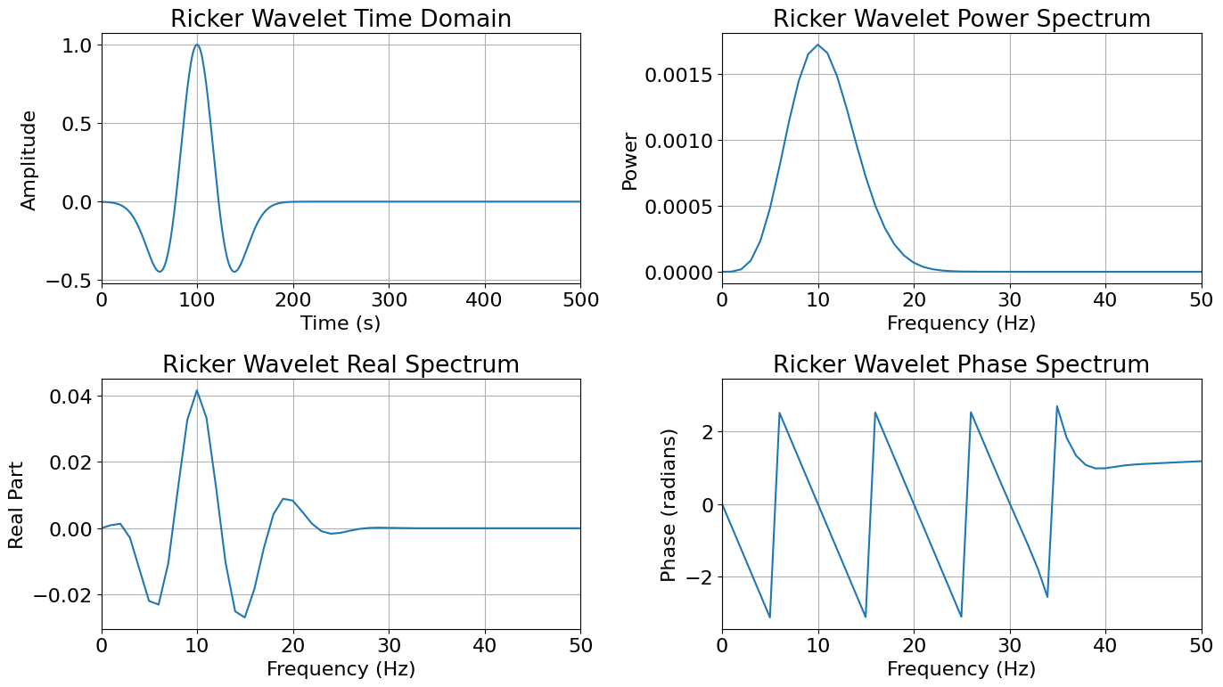
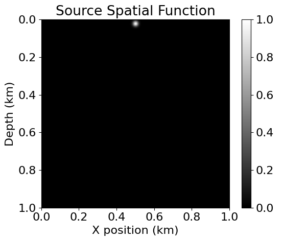
In this case, the acquisition geometry defines a predefined point source, but to simulate an extended source, we define a spatial distribution for the source:

# Source spatial distribution ------------
src_space = Function(name='src_space', grid=model.grid)

X, Z = np.meshgrid(
	np.linspace(0, model.grid.extent[0], model.grid.shape[0]),
	np.linspace(0, model.grid.extent[1], model.grid.shape[1])
	)

# Gaussian source
x0 = geometry.src_positions[0][1]+model.nbl*model.spacing[1]
z0 = geometry.src_positions[0][0]+model.nbl*model.spacing[0]
sigma = 10

src_space.data[:] = np.exp(-((X - x0)**2 + (Z - z0)**2) / (2 * sigma**2))
# ----------------------------------------

Time Solution

Next, we define the time-stepping stencil for solving the wave equation:

# Define the wavefield time function with 
# the size of the model and the time dimension
u = TimeFunction(
  name="u",
  grid=model.grid,
  time_order=2,
  space_order=2,
  save=geometry.nt
  )

# Define the PDE for wave propagation
pde = model.m * u.dt2 - u.laplace + model.damp * u.dt

# Compute the time update stencil
stencil = Eq(u.forward, solve(pde, u.forward))
stencil

$\displaystyle u(t + dt, x, y) = \frac{- \frac{- \frac{2.0 u(t, x, y)}{dt^{2}} + \frac{u(t - dt, x, y)}{dt^{2}}}{vp(x, y)} + \frac{\partial^{2}}{\partial x^{2}} u(t, x, y) + \frac{\partial^{2}}{\partial y^{2}} u(t, x, y) + \frac{damp(x, y) u(t, x, y)}{dt}}{\frac{damp(x, y)}{dt} + \frac{1}{dt^{2} vp(x, y)}}$

Then, we define the equations to compute the frequency modes and to inject the source into the wavefield. Finally, we create the operator that executes the time-stepping, producing the numerical solution of the wave equation and while simultaneously computing the frequency modes.

nfreq = 31 # number of frequencies
f = Dimension(name='f') # frequency dimension

# Define the frequencies we want to calculate
frequencies = Function(
	name='frequencies',
	dimensions=(f,),
	shape=(nfreq,),
	dtype=np.float32
	)
frequencies.data[:] = np.linspace(0.001, 0.03, nfreq)

# Define the DFT function to store the frequency domain wavefield
freq_modes = Function(
	name='freq_modes',
	grid=model.grid,
	space_order=0,
	dtype=np.complex64,
    dimensions=(f, *model.grid.dimensions), 
    shape=(nfreq, *model.grid.shape)
    )

# Define the On-the-Fly DFT equation
omega = 2 * np.pi * frequencies
basis = exp(-1j * omega * model.grid.time_dim * model.grid.time_dim.spacing)
dfts = [Inc(freq_modes, basis * u *dt*1e-3)]

# Inject the source into the wavefield
src_expr = src_space*geometry.src * dt**2 / model.m
eq_src = Eq(u.forward, u.forward + src_expr)
display(eq_src)

$\displaystyle u(t + dt, x, y) = 0.765275 vp(x, y) src_space(x, y) src(time, p_src) + u(t + dt, x, y)$

# Define the operator
op = Operator([stencil, eq_src] + dfts, subs=model.spacing_map)
u.data.fill(0)

# Execute the operator
op(dt=model.critical_dt)

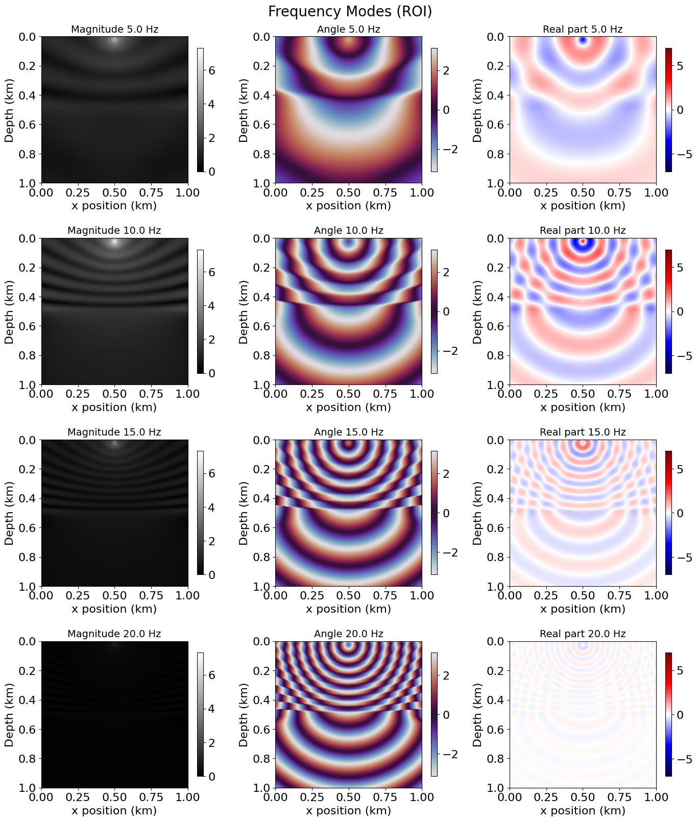
Frequency Domain

We plot several of the simulated frequency modes. As expected, their amplitudes vary according to the power spectrum of the source.

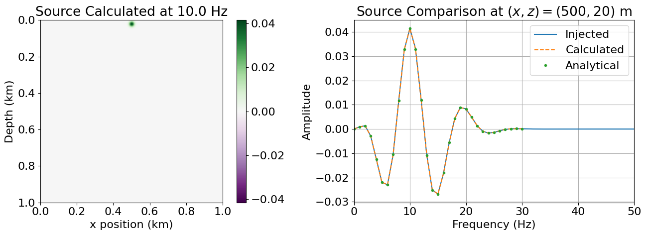
Source Spatial Analysis

Finally, we apply the differential operator of the Helmholtz equation to the solution to compute the effective source term. We then compare this result with the injected source (obtained via the Fourier transform of the original source) and the theoretical value. The comparison shows that the calculated and theoretical source terms correspond closely, validating the simulation.

References

F. Luporini et al., “Architecture and Performance of Devito, a System for Automated Stencil Computation,” ACM Trans. Math. Softw., vol. 46, no. 1, pp. 1–28, Mar. 2020, doi: 10.1145/3374916. ↩︎
M. Louboutin et al., “Devito (v3.1.0): an embedded domain-specific language for finite differences and geophysical exploration,” Geosci. Model Dev., vol. 12, no. 3, pp. 1165–1187, Mar. 2019, doi: 10.5194/gmd-12-1165-2019. ↩︎
Devito, “17 - On-the-fly discrete Fourier transform,” Tutorials, Seismic modeling and inversion. Accessed: Oct. 12, 2025. [Online]. Available: devitoproject.org ↩︎ ↩︎ ↩︎