An overview of Wave Propagation within Seismic Tomography

In this post, I provide an overview of seismic wave propagation within the seismic tomography geophysical imaging technique, based on several bibliographic resources I have studied.

What is a Seismic Wave?

Seismic waves are disturbances in Earth materials (media) that carry and propagate energy ¹. They are generated when a source of impulsive mechanical energy is initiated within an elastic medium ². The volume and shape changes oscillate about their neutral positions while simultaneously propagating away from the energy source. ². However, the medium itself in generally does not travel with the wave; once the disturbance has passed, the material usually returns to its original position and appearance, provided the medium is elastic ¹.

The passage of a seismic wave produces two main effects on the medium: redistribution of internal forces (stress changes) and modification of volume and geometrical shape (strain changes) ². Seismic energy sources can be natural, such as earthquakes, or artificial, such as dynamite explosions or mechanical devices ².

Types of Seismic Waves

Two types of seismic waves travel through the Earth’s interior, while two others spread out at and near its surface. Each type is characterized by distinct ground motions, and their speeds vary according to the elastic properties and density of the rocks they traverse.

Seismic Body Waves

Body waves are seismic waves that travel through an elastic medium in any direction. They are divided into two subtypes: longitudinal waves and transverse waves ².

P-waves (compressional, primary, or longitudinal waves)

P-waves cause particles in the medium to vibrate about their neutral positions in the direction of wave propagation, producing a “volume” deformation characterized by alternating compressions and expansions. They are the fastest type of seismic wave, so they are always the first to be detected at observation points. P-waves can even travel through liquids, although with reduced speed ^{2 3}.

S-waves (shear, secondary, or transverse waves)

S-waves, or secondary waves, involve particle motion that is transverse to the direction of propagation, resulting from shear strain or “shape” deformation of the medium. Because shear waves can only travel in a material that supports shear strain, S-waves cannot travel through fluids. They are slower than P-waves and therefore arrive later at observation points. Depending on their polarization, they are classified as SV-waves, with particle motion confined to a vertical plane, or SH-waves, with particle motion in a horizontal plane (parallel to the ground surface) ^{2 3}.

Seismic Surface Waves

Surface waves are waves that move on the free surface of the earth. Compared with body waves, they have relatively large amplitudes, lower frequencies, and slower velocities in the same medium ². On a seismogram, P-waves arrive first, followed by S-waves and then the surface waves ³. The principal types of surface waves are Rayleigh waves and Love waves.

Rayleigh Waves

Rayleigh waves develop along the free surface of a semi-infinite solid medium, with amplitudes that decay rapidly with depth. The travelling disturbance in this case is a sort of combination of particle-motions of both P- and SV-waves. The particle motion, which has a retrograde elliptical orbit, takes place in a vertical plane parallel to propagation direction ^{2 3}.

Love Waves

Love waves occur when a solid elastic semi-infinite medium is overlain by a horizontal low-velocity layer, which traps the horizontal components of shear waves between the free surface and the lower interface. The resulting motion is purely transverse, confined to the horizontal plane, and can generate intense horizontal ground shaking with significant effects on structures ^{2 3}.

Reflection, Refraction, and Diffraction of Body Waves

In the Earth Crust, a seismic wave may meet a variety of geological changes. Typically, the media are made up of layered rock formations of different densities and elastic properties, which changes the velocity of propagation. ² When a P- or S-wave hits the boundary between two materials it excites vibrations on both sides, and some of its energy is reflected back into the first medium and some is transmitted into the second. This process, which is governed by rules similar to those of light waves in optics, produces new seismic waves on either side of the interface ³.

Reflection

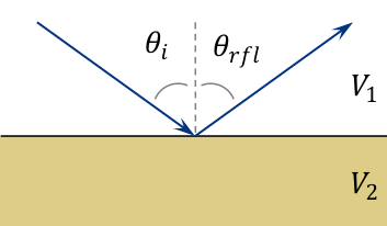
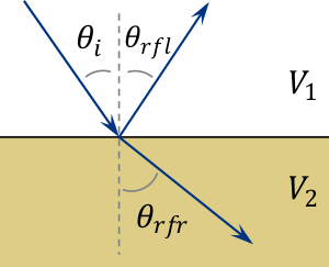
The angle between a ray and a normal to the horizontal surface is termed the angle of incidence $\theta_i$. The angle of incidence equals the angle of reflection $\theta_{rfl}$.

$$\theta_i=\theta_{rfl}, \quad \text{(Reflection)}.$$

Refraction

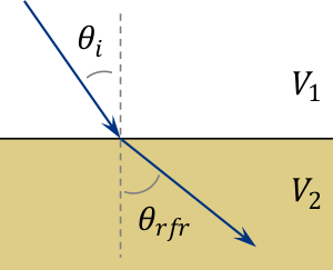
The rest of the incident wave is transmitted through the interfaces with their ray-paths being bent (refracted) in case of inclined incidence and with no bending when ray-path is perpendicular to an interface ⁴.

$$V_{rfr}  \sin⁡ \theta_i =V_i  \sin \theta_{rfr}, \quad \text{(Snell’s Law )}.$$

Critical refraction

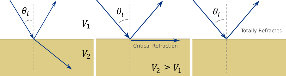
The angle of refraction increases as the angle of incidence increases until rays are refracted parallel to the interface between the two materials (critically refraction). If the angle of incidence increases beyond this special value, then no refraction occurs, and the ray is totally reflected ⁵.

$$\theta_{i_c}=\sin^{-1}⁡\left(V_1/V_2\right).$$

Head Waves: The critically refracted ray travels parallel to the interface, but in the $V_2$ medium, and produces a disturbance in $V_2$ at the $V_1/V_2$ interface. Because the $V_1$ material must move in phase with the $V_2$ material, there is a disturbance in the $V_1$ material moving at $V_2$. This generates secondary wavelets as the refracted wave passes, which return to the surface through the $V_1$ medium at velocity $V_1$ ⁵.

Diffraction

Seismic waves may be reflected at interfaces or diffracted by structural obstacles ⁴. Diffraction arises when a seismic wave encounters an abrupt or discontinuous surface, such as an intruding body or the edge of a layer ³. If a disturbance is generated at the surface and encounters a sudden change of curvature at a velocity discontinuity, additional waves are produced that we cannot predict by drawing rays for reflection or refraction ⁵. Diffraction will be most important when sharp changes in curvature have radii that are similar in dimension to seismic wavelengths ⁵.

Dispersion

Waveform distortion caused by the dependence of velocity on frequency components is known as dispersion. In a dispersive medium, each frequency component of a seismic wave travels at its own velocity, so a signal composed of multiple frequencies gradually separates into its components, altering its shape during propagation. The velocity of an individual frequency component (each wave-phase) is called the phase velocity, while the velocity of the wave packet as a whole, defined by the envelope of the wave train, is called the group velocity. Dispersion is most significant in surface waves. In contrast, dispersion of seismic body waves are too small to be detected in practice: their velocities remain nearly constant across a broad frequency range, the effect is so small that it is usually ignored in seismic exploration ².

Scattering

In a laterally homogeneous or slowly varying medium, seismic wavefronts can be perfectly tracked and wave propagation can be successfully described by geometrical methods such as ray theory. However, in the presence of obstacles, or lateral variations of elastic parameters, wavefronts are distorted and seismic energy can be deflected in all possible directions: a phenomenon known as wave scattering. The scattering of seismic waves is intimately related to the heterogeneous nature of Earth materials on a variety of spatial scales ⁶.

Wave conversion at interfaces

When a seismic wave hits an interface at an oblique angle, additional wave phases are generated. For instance, when a P-wave or SV-wave encounters the boundary between two solids with different densities and elastic properties (i.e., different acoustic impedances), four phases arise: reflected and refracted P-waves and SV-waves. In contrast, if the incident wave is an SH-wave, only reflected and refracted SH-waves are produced. The SV-waves generated from an incident P-wave, or the P-waves generated from an incident SV-wave, are known as converted waves ².

Seismic Tomography

Seismic tomography is an inversion technique that uses seismic data to construct models of the Earth’s subsurface, typically in terms of velocity and structural dimensions ². It has been widely applied to image seismic velocity variations and build detailed geological models ². By analyzing seismic wave travel-times along ray paths crossing a region from multiple directions, tomography reveals velocity contrasts within the Earth. Seismic tomography can be based on the travel-times of P-waves, S-waves, or surface waves. Other geophysical properties, such as attenuation, can also be investigated through amplitude modeling ^{2 3}.

Types of Seismic Tomography

Two main approaches are used: reflection tomography, which analyzes reflection travel-time measurements, and transmission tomography, which uses seismic transmission waves that experience refraction processes at boundaries where velocity changes. Transmission tomography requires putting the source points in a borehole and the receiver points at another borehole or at the surface ².

The Refraction Method

When the incident angle equals the critical angle $\theta_{i_c}$, a special refracted wave, called the head wave, is generated. This critically refracted wave travels along the interface with the velocity $V_2$ of the lower medium and is refracted back to the earth’s surface at the same angle $\theta_{i_c}$, propagating through the upper medium with velocity $V_1$ ⁷.

On seismic shooting records, three main wave arrivals are usually observed: direct waves, refracted waves, and reflected waves. The travel-time functions of the direct and refracted waves are linear, whereas that of the reflected wave is hyperbolic. At the critical distance $x_c$, where the incidence is at the critical angle, a head wave is generated. Between the source and $x_c$​, no refraction arrivals are observed, creating a shadow zone for refracted waves ⁷.

For a simple interface between two constant-velocity media, the refraction travel-time function is a straight line tangent to the reflection hyperbola at the point where both arrivals occur simultaneously. At small source-receiver distances, the direct wave arrives first because it follows the shortest path. Beyond the cross-over distance $x_{cr}$, the faster refraction wave overtakes the direct wave ⁷.

The velocities of the two layers can be calculated from the slopes of the linear travel-time functions, since velocity is the inverse of the slope of the time-distance line ⁷.

Seismic Noise

In seismology, the term noise refers to any disturbance that interferes with or masks the seismic signal of interest. What counts as noise depends on the focus of the study: when analyzing reflected body waves, surface waves, direct arrivals, and refractions are considered noise, while in refraction studies, reflected arrivals are treated as noise. In a stricter sense, however, ambient seismic disturbances (random background vibrations that overlay distinct traveling signals) are generally referred to as seismic noise ².

Coherent Noise

Coherent noise is a seismic event characterized by a distinct apparent velocity and well-defined onset. They are made up mainly of surface waves (ground roll) and air-waves which are of fairly narrow bandwidth with low frequency range ².

Incoherent Noise

Incoherent noise, in contrast, is random in both amplitude and onset. It forms the background energy present in any seismic record, in exploration seismology it is known as ambient noise. This type of noise has a broad frequency spectrum compared with the narrower bands of reflection signals or coherent noise. Terms such as white noise (broadband) and red noise (low-frequency) are sometimes used in geophysics to describe different forms of incoherent noise ².

Passive Sources

Active sources generate seismic waves using artificially created energy. In an active seismic reflection survey, a controlled source (such as explosives or a vibroseis truck) produces seismic energy, and the reflected signals are recorded to image subsurface structures ⁸.

Passive sources, in contrast, do not use artificial sources. Instead, they use natural seismic sources, such as microseisms and ambient seismic noise. Passive seismic methods record and analyze this background energy to image the subsurface in a relatively inexpensive and noninvasive way ⁸. They identify resonant frequencies and track changes over time. Typically, passive surveys employ three-component (3C) sensors and require long listening times, ranging from several hours to several days ⁹.

Forward and Inverse Modelling

Modeling processes are usually divided into two types: direct (forward) modeling and inverse modeling. The forward modeling, is based on assuming the geological model (its shape and physical properties), and then calculates the expected geophysical response. The inverse modeling, on the other hand is computing a model that can give a geophysical response which is closest to that observed ⁹.

Forward Modelling

Wave equation

The standard (acoustic) wave equation describes the strain-changes as function of space and time, expresses the variation of the disturbance $U$ (particle displacement or pressure field) as it propagates through a perfectly elastic medium ²:

$$\nabla^2 U = \frac{1}{c^2}\frac{d^2U}{dt^2},$$

where $c$ is the propagation velocity of the wave.

Helmholtz equation

For time-harmonic waves of the form

$$U(\textbf{r},t)=u(\textbf{r})e^{i\omega t},$$

with frequency $\omega>0$, the complex valued space dependent part $u$ satisfies the reduced wave equation or Helmholtz equation:

$$\nabla^2 u + k^2u = 0,$$

where the wave number $k$ is given by the positive constant $k = \omega/c$ ¹⁰.

Inverse Modelling

Full Wave Inversion

Full Waveform Inversion (FWI) is a seismic processing technique designed to produce quantitative subsurface models (physical property models, such as P-wave velocity) from seismic data. The principle is straightforward: the best model is the one whose synthetic shot gathers reproduce the observed data ¹¹.

In practice, however, FWI is a non-linear and iterative process, it requires an initial model. FWI simulates the physics of seismic wave propagation by solving the appropriate wave equation to generate synthetic wavefields and shot gathers, in order to mimic the physics of wave propagation ¹¹.

Two key aspects must be considered before applying FWI: (1) FWI uses the full wavefield (e.g., pressure field or vertical displacement at the receiver), rather than relying only on travel times and amplitudes. (2) FWI can provide high-resolution quantitative results if there is a correct understanding of the main phenomena influencing the wave propagation as well as a proper strategy to iteratively converge towards a meaningful solution ¹¹.

Classical and Deep Learning Frameworks

Devito ¹² is a Python package for implementing optimized stencil computations (e.g., finite differences) from high-level symbolic problem definitions. Built on SimPy, it uses automated code generation and just-in-time compilation to execute optimized computational kernels on several computer platforms, including CPUs, GPUs, and clusters. Devito is widely used to create wave propagation kernels for seismic inversion problems. The Seismic modeling and inversion tutorial provides a broad set of notebooks that implements various wave equations for modeling and inversion.

In parallel, recent research has explored physics-informed neural networks (PINNs) as an alternative approach to seismic modeling and inversion. Authors in ¹³ present an approach to the solution of the wave propagation and full waveform inversions (FWIs) based on PINNs. They present an algorithm applying PINNs to the acoustic wave equation, testing the method on both forward modeling and FWI case studies. Their results demonstrate that PINNs yield excellent results for inversions on all cases considered and with limited computational complexity ¹³.

References

M. M. Selim Saleh, “Body Waves,” in Encyclopedia of Solid Earth Geophysics, H. K. Gupta, Ed., Dordrecht: Springer Netherlands, 2011, pp. 29–35. doi: 10.1007/978-90-481-8702-7_140. ↩︎ ↩︎
H. N. Alsadi, “Seismic Waves,” in Seismic Hydrocarbon Exploration: 2D and 3D Techniques, H. N. Alsadi, Ed., Cham: Springer International Publishing, 2017, pp. 23–51. doi: 10.1007/978-3-319-40436-3_2. ↩︎ ↩︎ ↩︎ ↩︎ ↩︎ ↩︎ ↩︎ ↩︎ ↩︎ ↩︎ ↩︎ ↩︎ ↩︎ ↩︎ ↩︎ ↩︎ ↩︎ ↩︎ ↩︎ ↩︎ ↩︎
W. Lowrie, “Seismology and the Earth’s internal structure,” in Geophysics: A Very Short Introduction, W. Lowrie, Ed., Oxford University Press, 2018. doi: 10.1093/actrade/9780198792956.003.0003. ↩︎ ↩︎ ↩︎ ↩︎ ↩︎ ↩︎ ↩︎ ↩︎
H. N. Alsadi, “Seismic Wave Reflection and Diffraction,” in Seismic Hydrocarbon Exploration: 2D and 3D Techniques, H. N. Alsadi, Ed., Cham: Springer International Publishing, 2017, pp. 71–88. doi: 10.1007/978-3-319-40436-3_4. ↩︎ ↩︎
H. R. Burger, A. F. Sheehan, and C. H. Jones, Eds., “Seismic Exploration: Fundamental Considerations,” in Introduction to Applied Geophysics: Exploring the Shallow Subsurface, Cambridge: Cambridge University Press, 2023, pp. 7–64. doi: 10.1017/9781009433112.004. ↩︎ ↩︎ ↩︎ ↩︎
L. Margerin, “Seismic Waves, Scattering,” in Encyclopedia of Solid Earth Geophysics, H. K. Gupta, Ed., Dordrecht: Springer Netherlands, 2011, pp. 1210–1223. doi: 10.1007/978-90-481-8702-7_54. ↩︎
H. N. Alsadi, “Seismic Wave Transmission and Refraction,” in Seismic Hydrocarbon Exploration: 2D and 3D Techniques, H. N. Alsadi, Ed., Cham: Springer International Publishing, 2017, pp. 89–104. doi: 10.1007/978-3-319-40436-3_5. ↩︎ ↩︎ ↩︎ ↩︎
M. Naghizadeh et al., “Active and Passive Seismic Imaging of the Central Abitibi Greenstone Belt, Larder Lake, Ontario,” J. Geophys. Res. Solid Earth, vol. 127, no. 2, p. e2021JB022334, Feb. 2022, doi: 10.1029/2021JB022334. ↩︎ ↩︎
H. N. Alsadi, “Extra Exploration Tools,” in Seismic Hydrocarbon Exploration: 2D and 3D Techniques, H. N. Alsadi, Ed., Cham: Springer International Publishing, 2017, pp. 291–300. doi: 10.1007/978-3-319-40436-3_11. ↩︎ ↩︎
D. Colton and R. Kress, “The Helmholtz Equation,” in Inverse Acoustic and Electromagnetic Scattering Theory, D. Colton and R. Kress, Eds., Cham: Springer International Publishing, 2019, pp. 15–42. doi: 10.1007/978-3-030-30351-8_2. ↩︎
H. Chauris, “Full waveform inversion,” in Seismic imaging: a practical approach, EDP Sciences, 2021, pp. 123–146. doi: [10.1051/978-2-7598-2351-2.c007](EDP Open). ↩︎ ↩︎ ↩︎
F. Luporini et al., “Architecture and Performance of Devito, a System for Automated Stencil Computation,” ACM Trans Math Softw, vol. 46, no. 1, Apr. 2020, doi: 10.1145/3374916. ↩︎
M. Rasht-Behesht, C. Huber, K. Shukla, and G. E. Karniadakis, “Physics-Informed Neural Networks (PINNs) for Wave Propagation and Full Waveform Inversions,” J. Geophys. Res. Solid Earth, vol. 127, no. 5, p. e2021JB023120, 2022, doi: 10.1029/2021JB023120. ↩︎ ↩︎